Relay FM — In Numbers

After doing The Incomparable, I had to go see what I could do with Relay FM’s data as well, naturally. So this is the beginning of that. The source code is included in this repo, and, in case anyone asks: Yes, you can use these graphs for whatever. Maybe link back to me, that would be cool.

Please note that there’s probably still stuff coming.

Overview

lastyear <- relay_episodes |>
  filter(year == year(now()) - 1) |>
  nrow()
thisyear <- relay_episodes |>
  filter(year == year(now())) |>
  nrow()
progress <- round(thisyear / lastyear * 100, 1)

Relay FM spans 48 shows and a combined runtime of over 399 days spread across 8677 episodes since 2014.

In 2025, there were 486 episodes published, and we’re currently about 39.3% of the way there at 191 episodes this year.

Shows by age

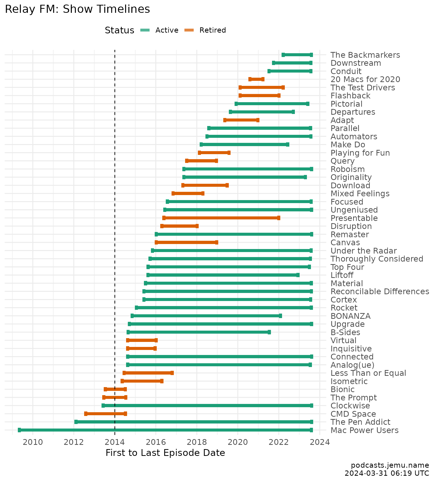
relay_episodes |>
  group_by(show) |>
  mutate(
    d_min = min(date),
    d_max = max(date)
  ) |>
  ggplot(aes(y = reorder(show, d_min), color = show_status)) +
  geom_errorbar(aes(xmin = d_min, xmax = d_max),
    width = .5, linewidth = 2, alpha = .85
  ) +
  geom_vline(xintercept = as.Date("2014-01-01"), linetype = "dashed", color = "grey60") +
  scale_x_continuous(
    transform = c("date", "reverse"),
    breaks = scales::breaks_width("2 years"),
    minor_breaks = scales::breaks_width("1 year"),
    labels = scales::label_date("%Y")
  ) +
  scale_color_manual(values = c(Active = "#009E73", Retired = "#999999")) +
  theme_relayfm() +
  theme(axis.text.y = element_text(hjust = 1)) +
  labs(
    y = NULL, x = "First to last episode date",
    title = "Relay FM: show timelines",
    caption = caption, color = "Status"
  )

Shows per year

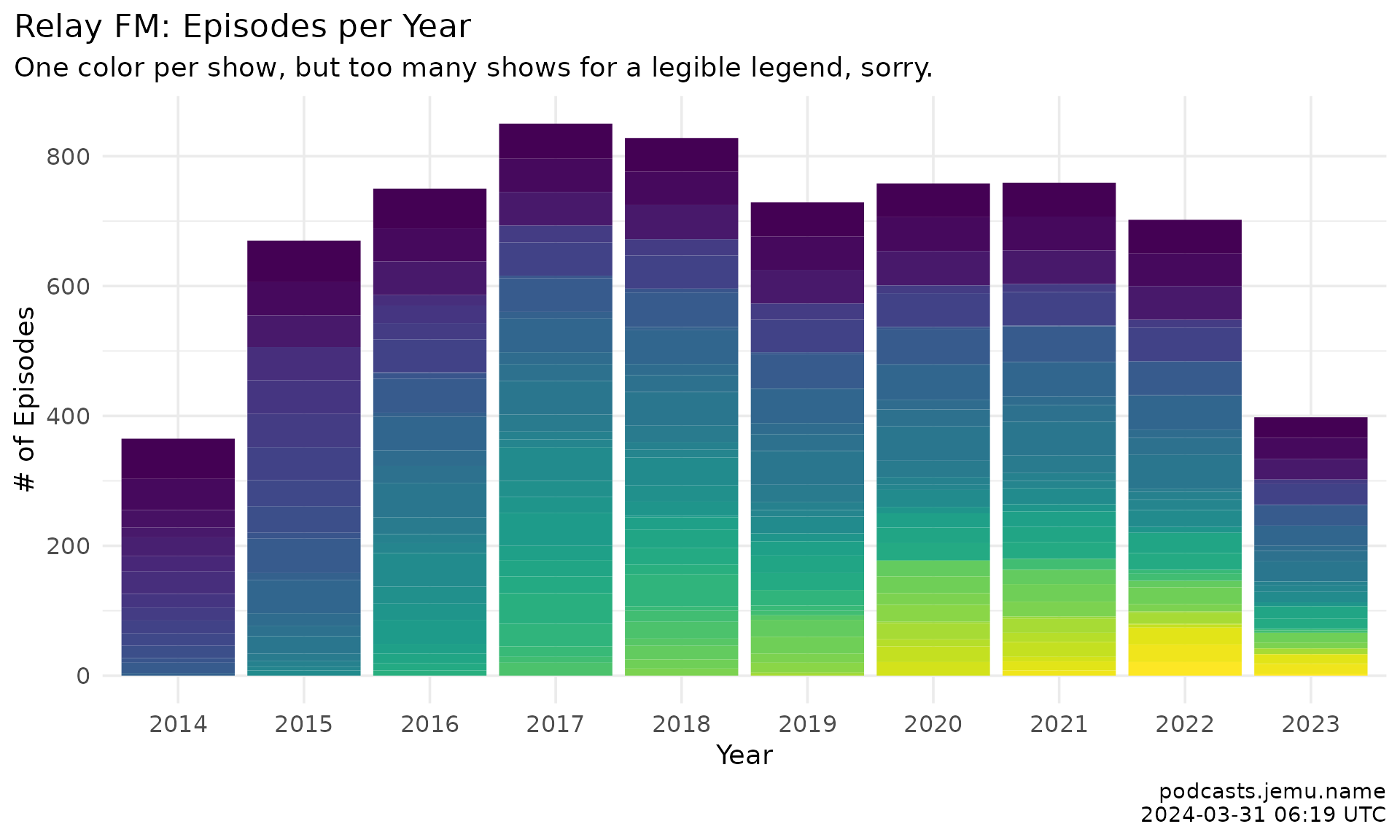
relay_episodes |>
  filter(year >= 2014) |>
  group_by(show, year) |>
  tally() |>
  ggplot(aes(x = as.factor(year), weight = n, fill = show)) +
  geom_bar(show.legend = FALSE) +
  scale_y_continuous(
    breaks = seq(0, 1e6, 200),
    minor_breaks = seq(0, 1e6, 100)
  ) +
  scale_fill_viridis_d(option = "mako") +
  theme_relayfm() +
  labs(
    x = "Year", y = "Episodes", fill = NULL,
    title = "Relay FM: episodes per year",
    subtitle = "One color per show; legend omitted at this many shows.",
    caption = caption
  )

Shows per week

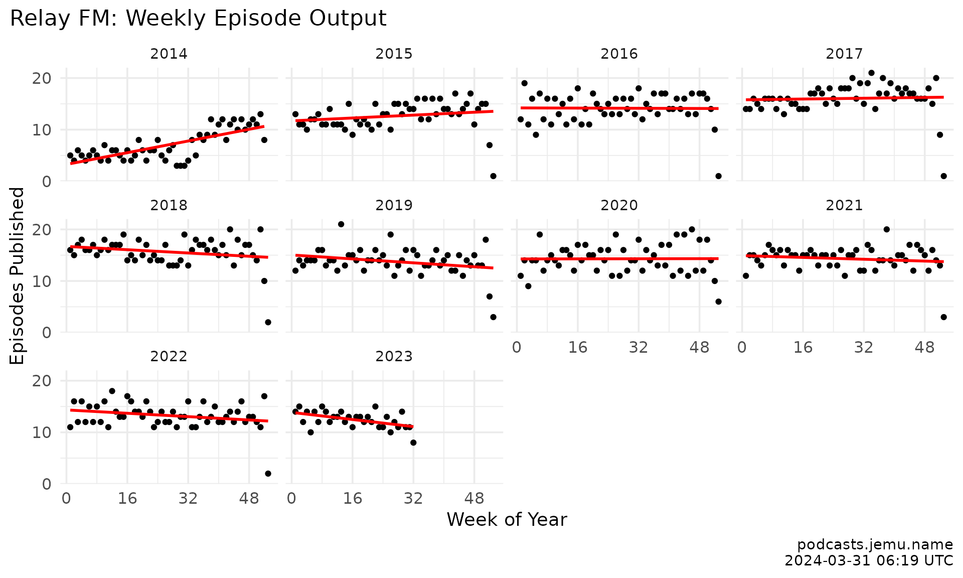
relay_episodes |>
  mutate(
    week = week(date),
    year_num = year(date)
  ) |>
  filter(year_num >= 2014) |>
  group_by(year, week) |>
  tally() |>
  ggplot(aes(x = week, y = n)) +
    geom_point(color = palette_relayfm[["slate"]], alpha = .6, size = 1.2) +
    geom_smooth(method = lm, formula = y ~ x, se = FALSE,
                color = relay_anchor, linewidth = 0.8) +
    scale_y_continuous(
      breaks = seq(0, 100, 10),
      minor_breaks = seq(0, 100, 5)
    ) +
    scale_x_continuous(breaks = seq(0, 55, 16)) +
    facet_wrap(~year) +
    theme_relayfm() +
    labs(
      title = "Relay FM: weekly episode output",
      x = "Week of year", y = "Episodes published",
      caption = caption
    )

Regularity (TBA)

relay_episodes |>
  mutate(
    week = isoweek(date),
    year_num = year(date)
  ) |>
  filter(year_num == current_year) |>
  count(show, year, week) |>
  ggplot(aes(x = week, y = n)) +
  geom_col(fill = palette_relayfm[["slate"]]) +
  facet_wrap(~show, ncol = 3, scales = "free") +
  theme_relayfm() +
  labs(
    title = "Relay FM", subtitle = "Episodes per week in the current year",
    x = "Week of year", y = "Episodes", caption = caption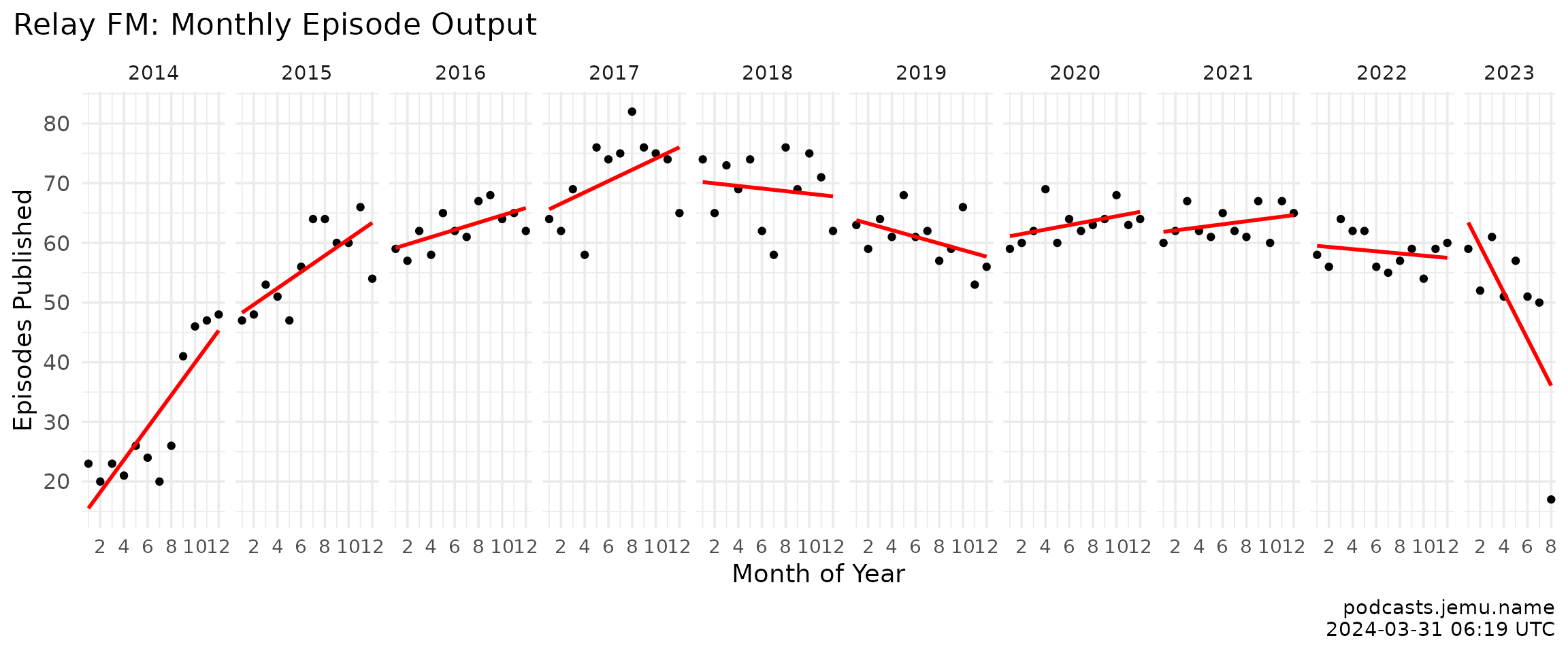
  )

Shows per month

relay_episodes |>
  mutate(
    month = month(date),
    year_num = year(date)
  ) |>
  filter(year_num >= 2014) |>
  count(year, month) |>
  ggplot(aes(x = month, y = n)) +
    geom_point(color = palette_relayfm[["slate"]], alpha = .6, size = 1.2) +
    geom_smooth(method = lm, formula = y ~ x, se = FALSE,
                color = relay_anchor, linewidth = 0.8) +
    scale_y_continuous(
      breaks = seq(0, 1e6, 10),
      minor_breaks = seq(0, 1e6, 5)
    ) +
    scale_x_continuous(
      breaks = seq(0, 13, 2),
      minor_breaks = seq(0, 13, 1)
    ) +
    facet_grid(. ~ year, space = "free_x", scales = "free_x") +
    theme_relayfm() +
    labs(
      title = "Relay FM: monthly episode output",
      x = "Month of year", y = "Episodes published",
      caption = caption
    )

Runtimes

All shows

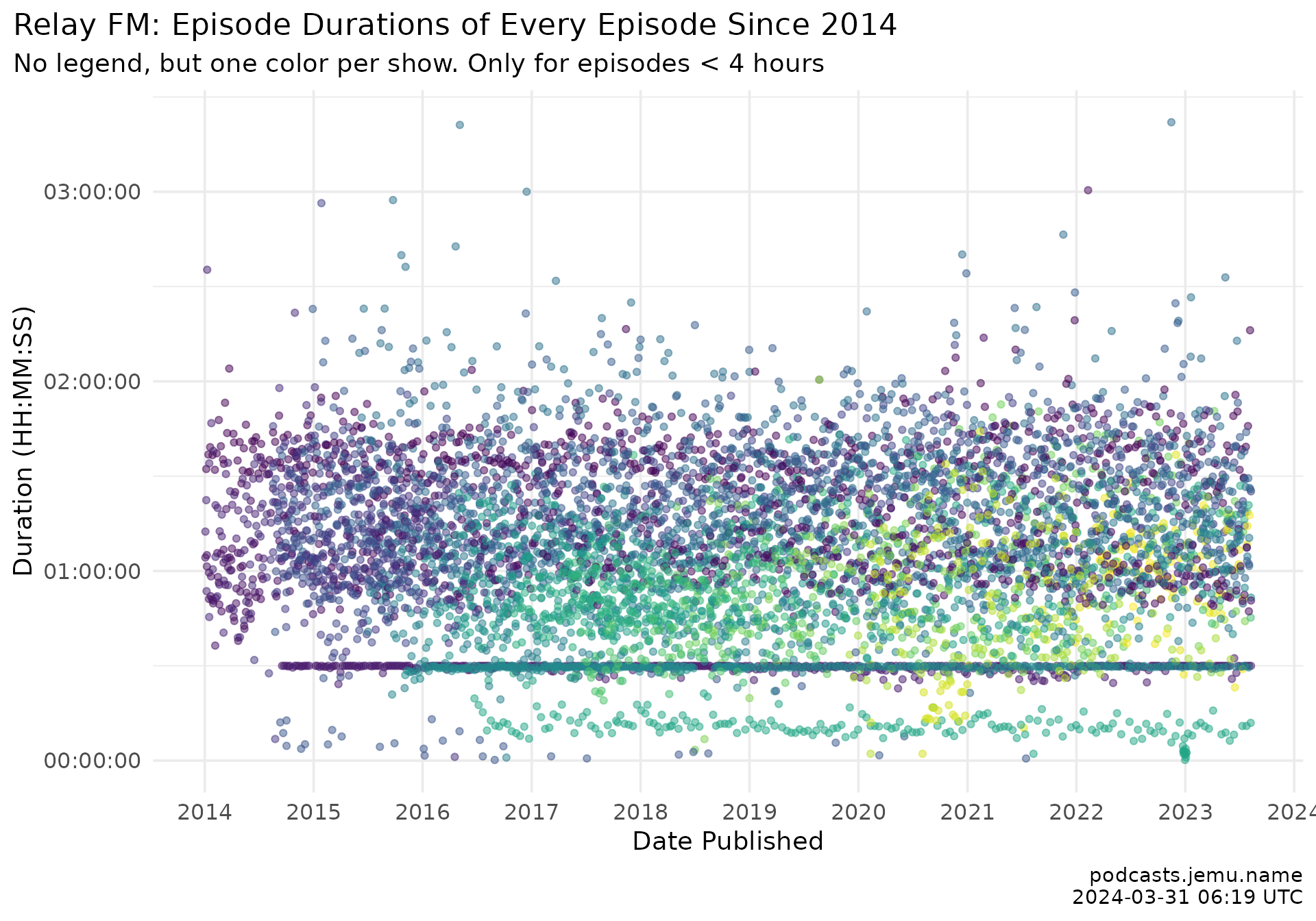
relay_episodes |>
  filter(year >= 2014, duration <= hms::hms(hours = 4)) |>
  ggplot(aes(x = date, y = duration, color = show)) +
  geom_point(alpha = .5, show.legend = FALSE, size = 1.2) +
  scale_x_date(
    date_breaks = "1 years",
    date_labels = "%Y",
    minor_breaks = NULL
  ) +
  scale_y_time(
    breaks = hms::hms(hours = seq(0, 1e6, 1)),
    limits = c(0, NA)
  ) +
  scale_color_viridis_d(option = "mako") +
  theme_relayfm() +
  labs(
    title = "Relay FM: episode durations since 2014",
    subtitle = "One color per show, no legend. Episodes under 4 hours only.",
    x = "Date published", y = "Duration (HH:MM:SS)",
    caption = caption
  )

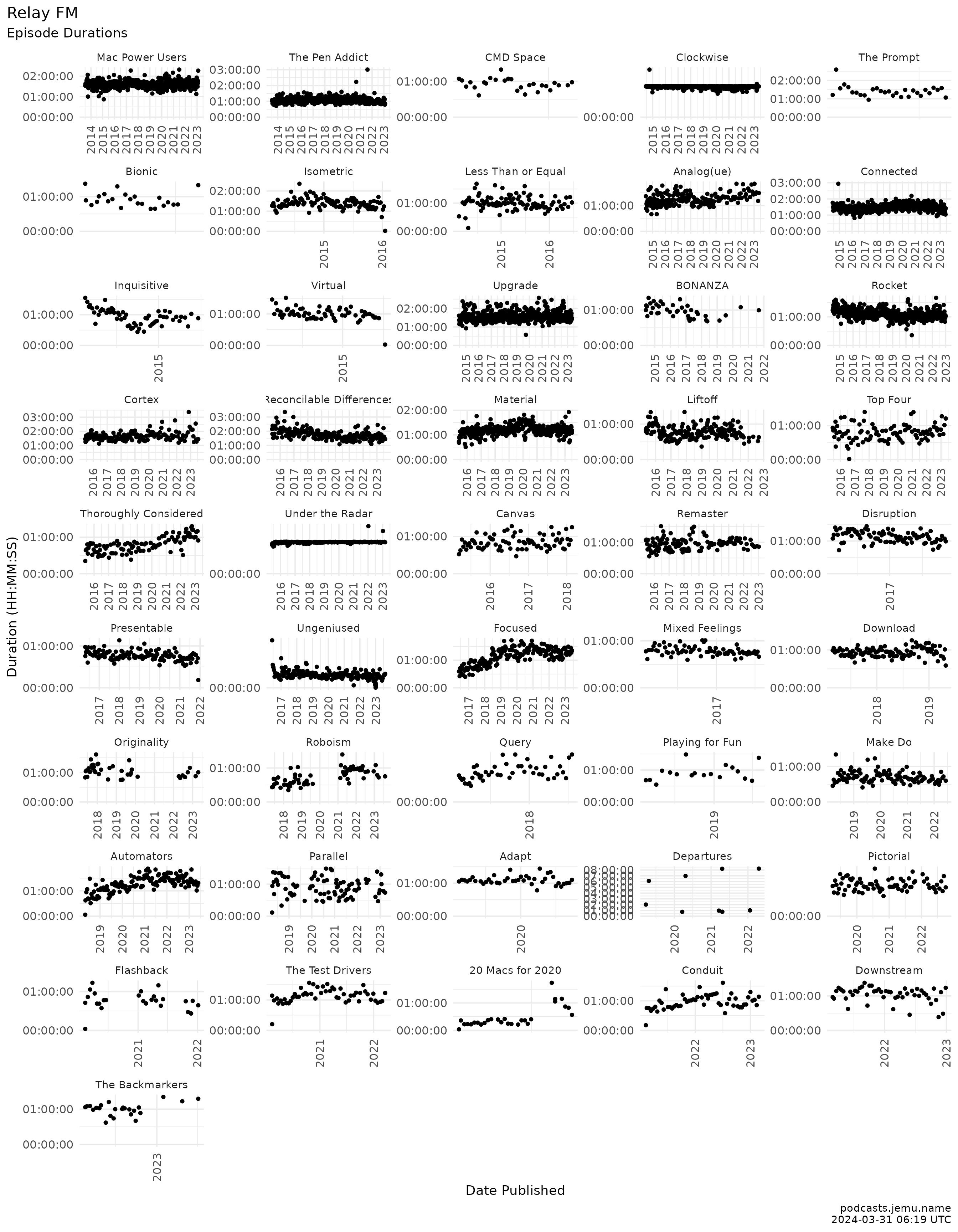
relay_episodes |>
  filter(show != "B-Sides", year >= 2014) |>
  ggplot(aes(x = date, y = duration)) +
    geom_point(color = palette_relayfm[["slate"]], alpha = .5, size = 1) +
    expand_limits(y = 0) +
    scale_x_date(
      date_breaks = "12 months",
      date_minor_breaks = "6 month",
      date_labels = "%Y"
    ) +
    scale_y_time(
      breaks = hms::hms(minutes = seq(0, 1e6, 60))
    ) +
    facet_wrap(~show, ncol = 5, scales = "free") +
    theme_relayfm() +
    theme(axis.text.x = element_text(angle = 90, vjust = .5)) +
    labs(
      title = "Relay FM: episode durations by show",
      x = "Date published", y = "Duration (HH:MM:SS)",
      caption = caption
    )

Histogram

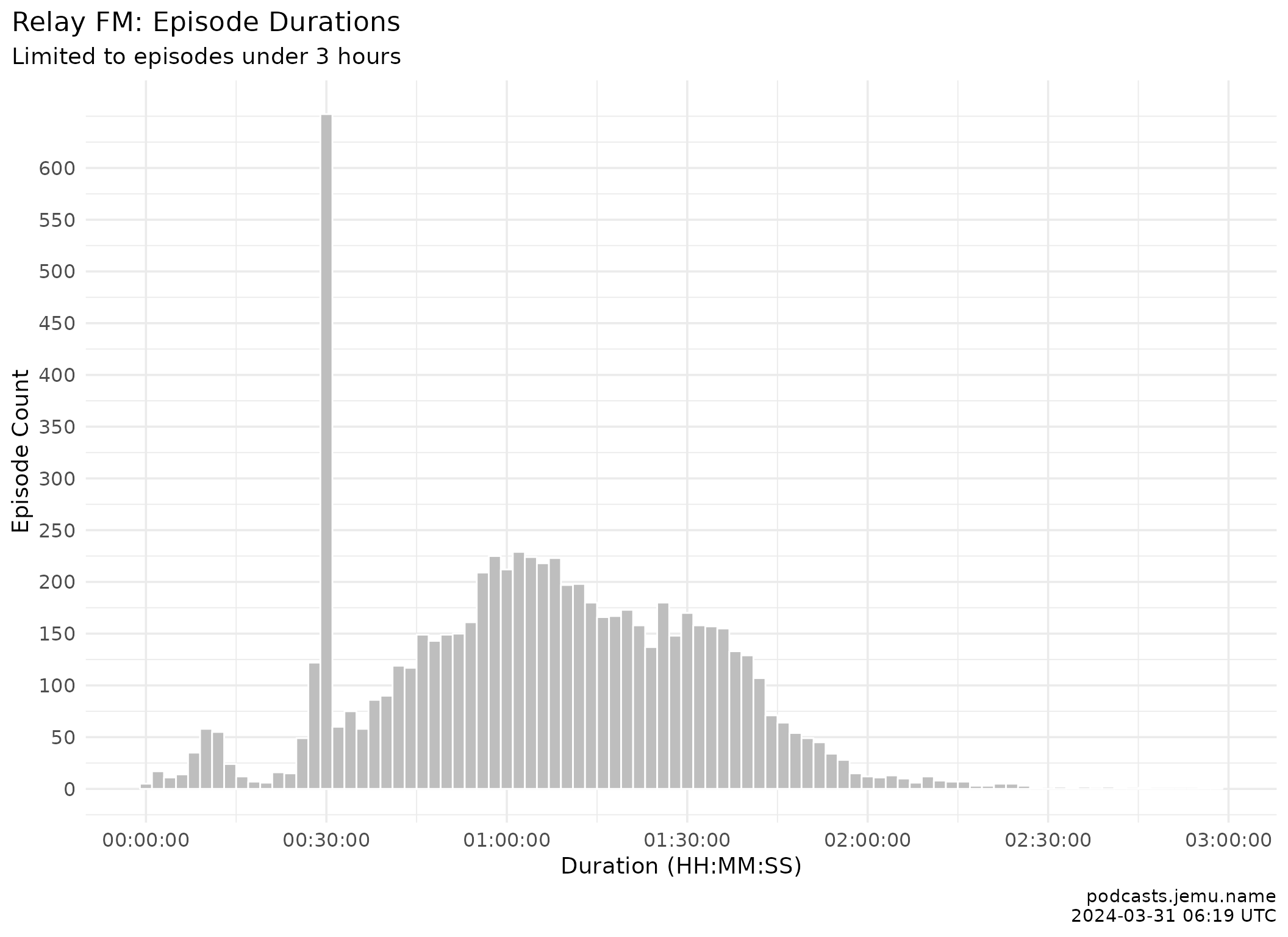
relay_episodes |>
  filter(duration <= hms::hms(hours = 3)) |>
  ggplot(aes(x = duration)) +
  geom_histogram(binwidth = 120,
                 fill = palette_relayfm[["slate"]], color = "white") +
  scale_x_time(
    breaks = hms::hms(minutes = seq(0, 1e6, 30))
  ) +
  scale_y_continuous(breaks = seq(0, 600, 50)) +
  theme_relayfm() +
  labs(
    title = "Relay FM: episode durations",
    subtitle = "Episodes under 3 hours.",
    y = "Episode count", x = "Duration (HH:MM:SS)",
    caption = caption
  )

Average by show

Boxplots

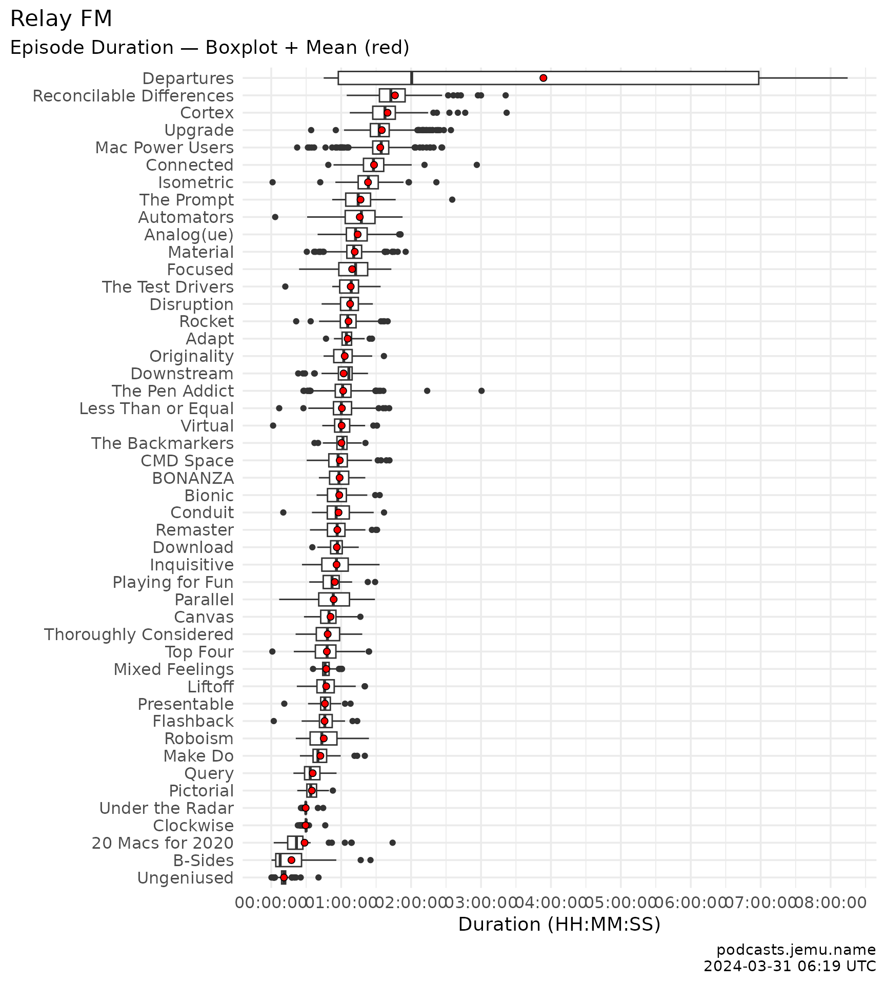
relay_episodes |>
  group_by(show) |>
  ggplot(aes(x = forcats::fct_reorder(show, duration, .fun = mean), y = duration)) +
    geom_boxplot(color = "grey25", fill = "grey95", outlier.size = 0.8) +
    stat_summary(
      fun = "mean", geom = "point", size = 2,
      color = relay_anchor
    ) +
    coord_flip() +
    scale_y_time(
      breaks = hms::hms(minutes = seq(0, 1e6, 60)),
      labels = scales::label_time(format = "%H:%M")
    ) +
    theme_relayfm() +
    labs(
      title = "Relay FM: episode duration by show",
      subtitle = "Boxplot per show; show mean marked in blue.",
      x = NULL, y = "Duration (H:M)",
      caption = caption
    )

People

Sadly I don’t have a lot of data about people besides the hosts of each show. I could try to pry out the guests of shows out of each show’s RSS feed, but sadly this information is not neatly presented in the feed, but rather would require an amount of regexing I am not prepared, and therefore not able to do. Be that as it may, here’s a bit about the hosts.

relay_episodes |>
  poddr::gather_people() |>
  count(person) |>
  ggplot(aes(x = reorder(person, n), y = n)) +
  geom_col(fill = palette_relayfm[["slate"]]) +
  coord_flip() +
  theme_relayfm() +
  labs(
    title = "Relay FM: hosts by episode count",
    x = NULL, y = "Episodes hosted",
    caption = caption
  )

Host by hours per week of podcasting

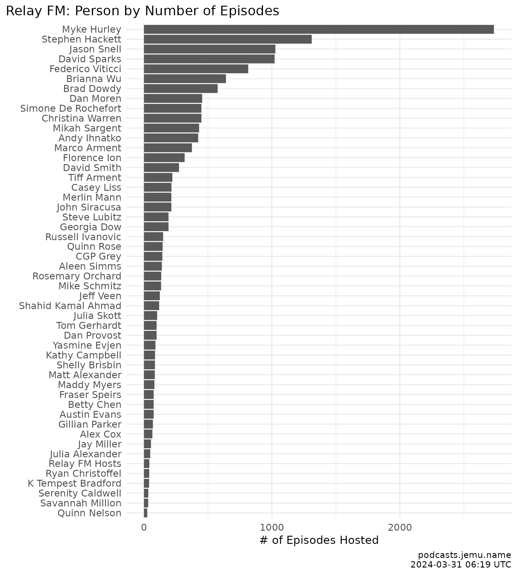
Filtered to episodes airing in 2014 or later.

relay_episodes |>
  filter(year >= 2014) |>
  poddr::gather_people() |>
  group_by(person) |>
  summarize(
    n = n(),
    duration = sum(duration, na.rm = TRUE),
    first_show = min(date, na.rm = TRUE),
    last_show = max(date, na.rm = TRUE),
    weeks_active = first_show %--% last_show / lubridate::dweeks(1),
    duration_per_week = as_hms(duration / weeks_active),
    .groups = "drop"
  ) ->
  people_activity


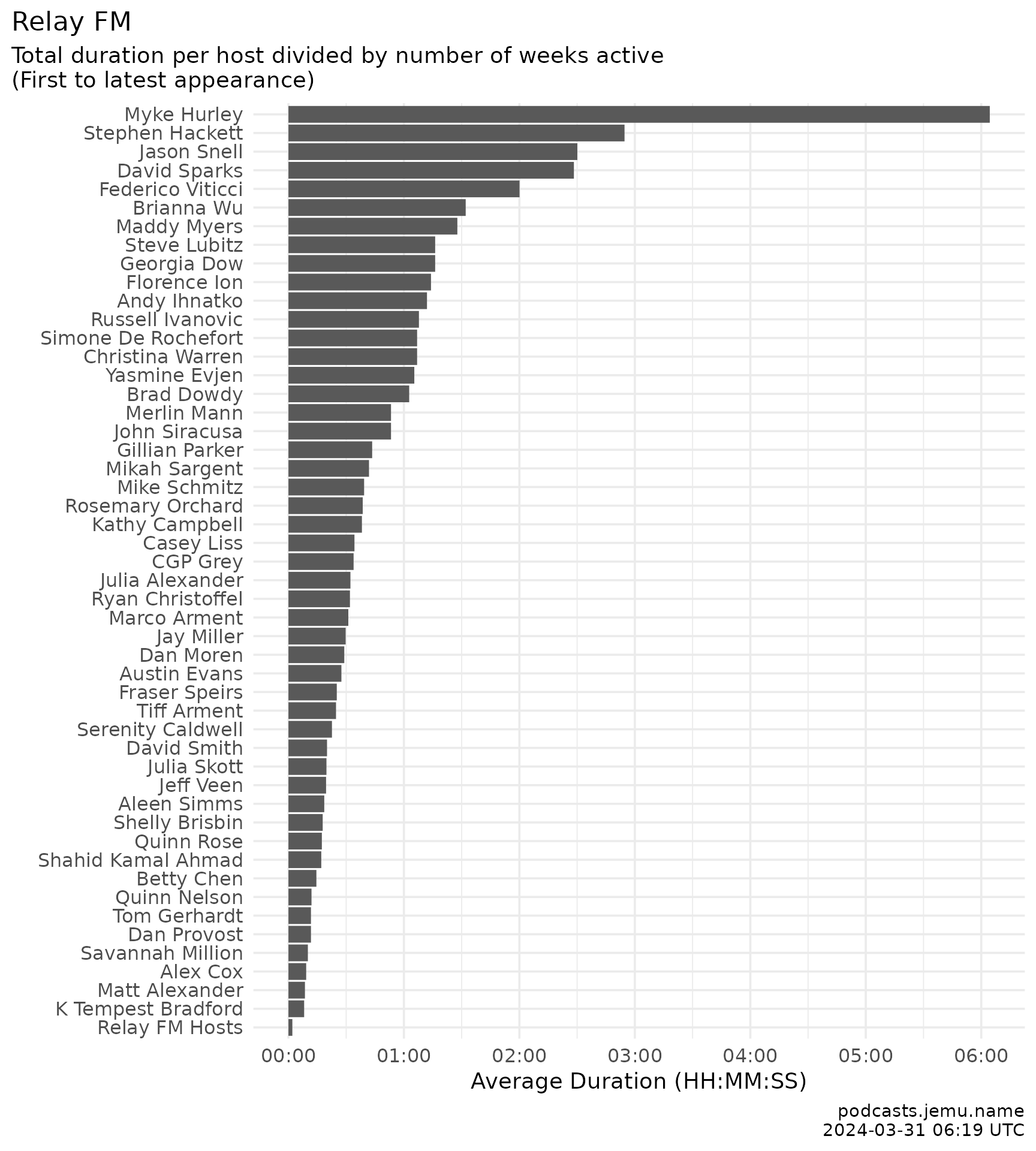
ggplot(people_activity, aes(x = reorder(person, duration_per_week), y = duration_per_week)) +
  geom_col(fill = palette_relayfm[["slate"]]) +
  coord_flip() +
  scale_y_time(
    breaks = hms::hms(minutes = seq(0, 1e6, 60)),
    labels = \(x) stringr::str_extract(as.character(x), "\\d{2}:\\d{2}")
  ) +
  theme_relayfm() +
  labs(
    title = "Relay FM: hours of podcast per active week",
    subtitle = "Total hosting duration divided by weeks from first to most recent appearance.",
    x = NULL, y = "Average duration (HH:MM:SS)",
    caption = caption
  )

Period of host activity

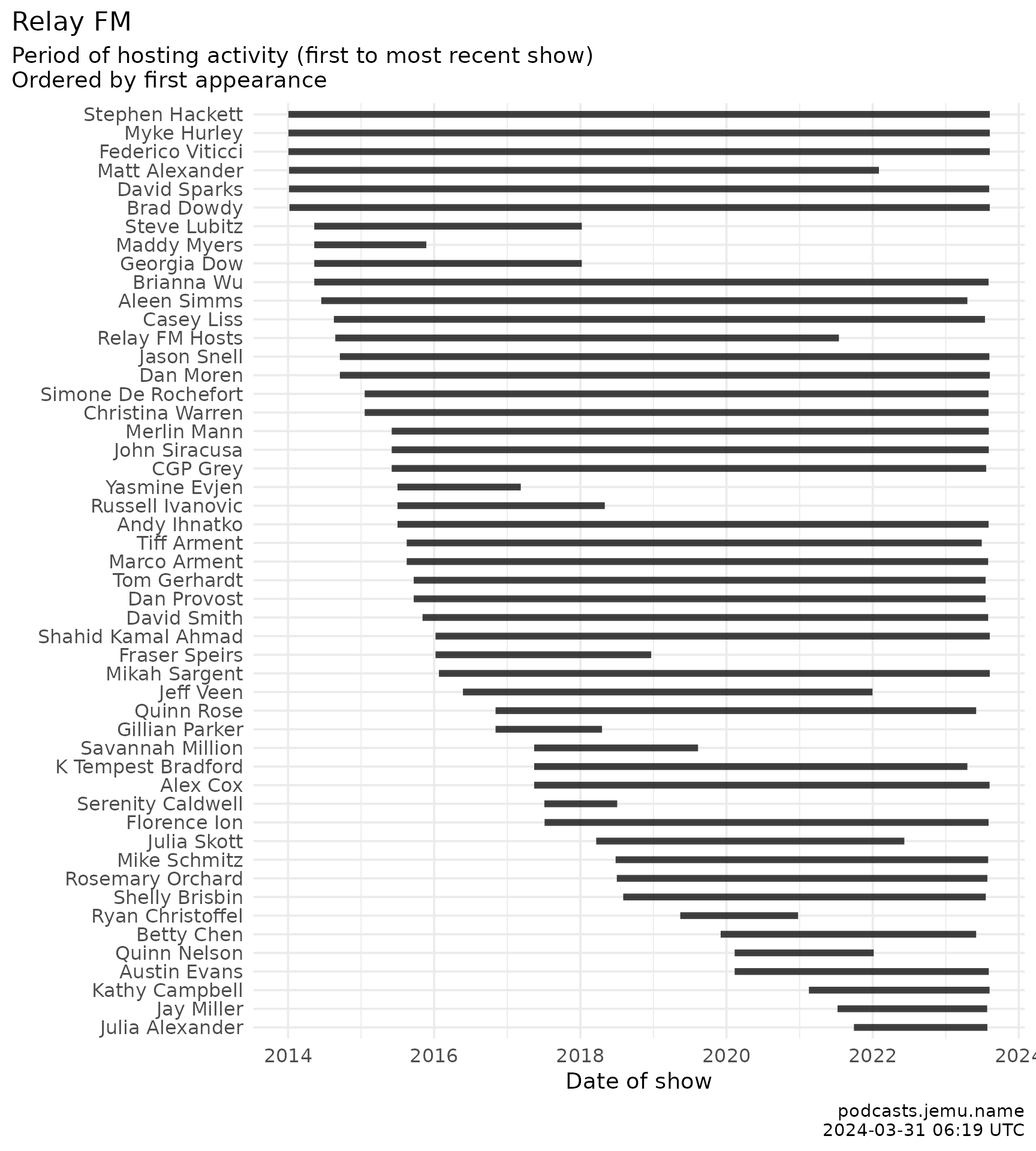
ggplot(people_activity) +
  geom_segment(aes(
    x = forcats::fct_reorder(person, first_show, .desc = TRUE), xend = person,
    y = first_show, yend = last_show
  ),
  linewidth = 2, alpha = .85, color = palette_relayfm[["slate"]]
  ) +
  coord_flip() +
  theme_relayfm() +
  labs(
    title = "Relay FM: period of hosting activity",
    subtitle = "First to most recent show; ordered by first appearance.",
    x = NULL, y = "Date of show",
    caption = caption
  )